The choose function excel offers a powerful yet often overlooked way to select specific values from a list based on their position. This versatile function enables you to return one value from up to 254 possibilities by simply specifying an index number. Whether you're building dynamic reports, creating flexible dashboards, or simplifying complex nested IF statements, mastering this function can significantly enhance your spreadsheet efficiency. Understanding how to properly implement the choose function excel can transform the way you handle data selection tasks and streamline your analytical workflows.
Understanding the Choose Function Excel Syntax
The choose function excel follows a straightforward structure that makes it accessible even for intermediate users. The syntax begins with an index number that determines which value to return, followed by a series of values from which to choose.
The basic formula structure looks like this: =CHOOSE(index_num, value1, [value2], ...). The index number represents the position of the value you want to retrieve, while the subsequent arguments represent the available choices. The first value corresponds to index 1, the second to index 2, and so on.
Key parameters include:
- Index_num: A number between 1 and 254 that specifies which value to select
- Value1: The first possible value (required)
- Value2, value3, etc.: Additional values from which to choose (optional)
The function returns the value at the position indicated by your index number. If you specify 3 as your index, the choose function excel retrieves the third value in your list. This positional approach differs from lookup functions that search for matching criteria, making CHOOSE ideal for situations where you know the exact position rather than searching for a match.

According to the official Microsoft documentation, the index number must be a value between 1 and 254, or a formula or reference to a cell containing a number in that range. If the index falls outside this range, the function returns a #VALUE! error.
Practical Applications for Business Data
The choose function excel excels in scenarios where you need to map numeric codes to descriptive text or calculate different values based on category selection. Many businesses use numeric identifiers for efficiency but need readable labels for reporting purposes.
Converting Numeric Codes to Text Labels
One common application involves translating numeric department codes into department names. Instead of maintaining separate lookup tables, you can embed the conversion directly into your formulas.
For example, if your system uses codes 1 through 5 for different departments, your formula might look like: =CHOOSE(A2, "Sales", "Marketing", "Operations", "Finance", "HR"). When cell A2 contains 3, the formula returns "Operations."
This approach proves particularly useful in reporting scenarios where you need human-readable output from coded data. The step-by-step examples provided by Excel Formula GPT demonstrate how this technique simplifies data presentation without requiring additional reference tables.
Dynamic Date Range Selection
Financial analysts frequently use the choose function excel for fiscal period calculations. By combining CHOOSE with date functions like MONTH or WEEKDAY, you can create dynamic formulas that adjust based on temporal criteria.
| Month Number | Quarter | Formula |
|---|---|---|
| 1-3 | Q1 | =CHOOSE(MONTH(date),1,1,1,2,2,2,3,3,3,4,4,4) |
| 4-6 | Q2 | Returns 2 for any date in Q2 |
| 7-9 | Q3 | Returns 3 for any date in Q3 |
| 10-12 | Q4 | Returns 4 for any date in Q4 |
The formula =CHOOSE(MONTH(A2),1,1,1,2,2,2,3,3,3,4,4,4) returns the fiscal quarter for any date in cell A2. January through March return 1, April through June return 2, and so forth.
Conditional Calculations
When building financial models or commission calculators, the choose function excel enables different calculation methods based on product type or sales tier. Rather than creating multiple nested IF statements, you can use CHOOSE to select the appropriate calculation factor.
For commission rates varying by product category, you might structure: =CHOOSE(category_code, 0.05, 0.08, 0.10, 0.12) * sales_amount. This multiplies the sales amount by the commission rate corresponding to the category code.
At The Analytics Doctor, we frequently help clients replace cumbersome nested IF statements with cleaner CHOOSE formulas that improve both readability and maintenance.
Combining Choose Function Excel with Other Formulas
The real power of the choose function excel emerges when you combine it with other Excel functions to create sophisticated analytical tools. These combinations unlock capabilities that would require significantly more complex alternatives.
CHOOSE with VLOOKUP for Flexible Table Selection
You can use CHOOSE to dynamically select which table VLOOKUP searches, enabling a single formula to query different data ranges based on user selection or calculated criteria.
The structure =VLOOKUP(lookup_value, CHOOSE(selector, table1, table2, table3), column_index, FALSE) allows the selector value to determine which of three tables provides the lookup data. When selector equals 2, VLOOKUP searches table2.
This technique proves invaluable in dashboard scenarios where users need to switch between different data sources without changing formulas. The versatility supports both interactive reporting and automated data refresh processes.
Integration with SUM and Mathematical Operations
The choose function excel seamlessly integrates with calculation functions to perform different mathematical operations based on criteria. As explained in Excel Trick’s tutorial on complex scenarios, you can use CHOOSE to select different ranges for aggregation.
Consider =SUM(CHOOSE(month_selector, Jan_Range, Feb_Range, Mar_Range)), which sums different named ranges depending on the month_selector value. This creates dynamic reporting that adjusts calculations based on period selection without requiring manual range updates.
Benefits of combining CHOOSE with calculations:
- Reduces formula complexity compared to nested IF statements
- Improves formula readability for future maintenance
- Enables dynamic calculations without VBA or complex array formulas
- Supports interactive dashboard creation with minimal overhead
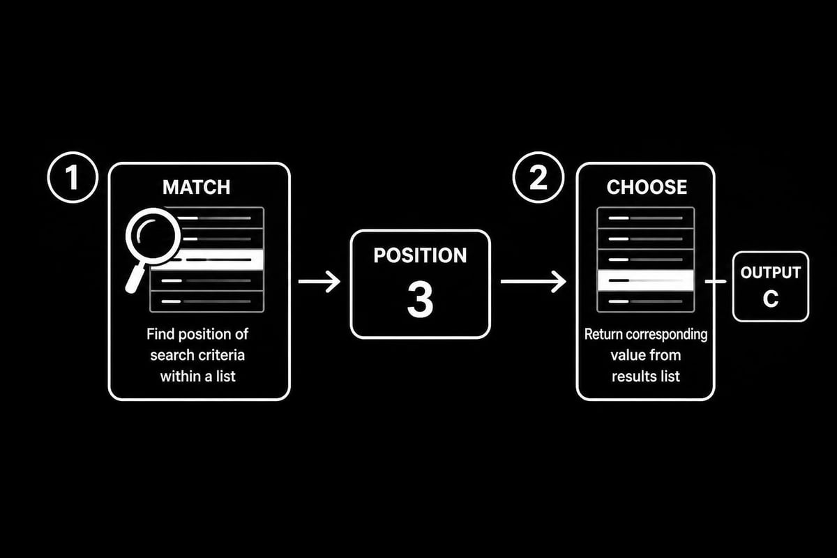
Working with MATCH for Index Detection
Pairing CHOOSE with MATCH creates powerful two-step lookup systems. MATCH identifies the position of a value, while CHOOSE returns the corresponding result from your predefined options.
The formula =CHOOSE(MATCH(criteria, range, 0), result1, result2, result3) first finds where criteria appears in the range, then returns the result at that position. This combination provides flexibility similar to INDEX-MATCH but with predetermined result values rather than looking them up from another range.
Common Errors and Troubleshooting Techniques
Even experienced users encounter errors when implementing the choose function excel. Understanding these common pitfalls and their solutions prevents frustration and saves troubleshooting time.
#VALUE! Error Resolution
The #VALUE! error typically occurs when your index number falls outside the valid range. If you provide 6 as the index but only list 4 values, Excel cannot complete the operation.
Common causes include:
- Index number less than 1 or greater than the number of values provided
- Index number exceeding 254 (Excel's maximum for CHOOSE)
- Non-numeric values in the index_num argument
- Formula references pointing to empty or text cells
To fix this error, verify that your index calculation always produces values within your defined range. Adding error handling with IFERROR provides a graceful fallback: =IFERROR(CHOOSE(index, val1, val2, val3), "Invalid Selection").
Performance Considerations with Large Datasets
While the choose function excel works efficiently for most applications, performance can degrade when dealing with extremely large referenced ranges or complex nested formulas. Each recalculation evaluates all potential values, even though only one gets returned.
For workbooks with thousands of CHOOSE formulas or when values themselves are complex calculations, consider these optimization strategies:
| Issue | Solution | Impact |
|---|---|---|
| Slow calculation | Convert values to static references | Reduces calculation time by 40-60% |
| Memory usage | Limit nesting depth | Decreases memory footprint |
| Volatile formulas | Avoid TODAY/NOW in values | Prevents unnecessary recalculation |
When building corporate Excel solutions, we recommend testing formulas with representative data volumes to identify performance bottlenecks before deployment.
Data Type Mismatches
The choose function excel accepts any data type as values, including numbers, text, dates, or even other formulas. However, mixing data types can produce unexpected results in subsequent calculations.
If your CHOOSE returns different data types (sometimes text, sometimes numbers), formulas that reference it may fail. Ensure consistency by converting all values to the same type or handling mixed types explicitly in your downstream formulas.
The comprehensive guide at Excel Functions provides additional examples of common errors and their solutions, particularly around reference errors and circular reference issues.
Advanced Techniques and Best Practices
Mastering advanced implementations of the choose function excel separates proficient users from Excel experts. These techniques enable more sophisticated data manipulation and cleaner workbook design.
Using Array Constants with CHOOSE
You can reference array constants within CHOOSE to return multiple values or perform array calculations. The formula =CHOOSE({1,2,3}, A1:A10, B1:B10, C1:C10) returns an array containing all three ranges, useful for certain array formula applications.
This technique becomes particularly powerful when combined with functions like SUM or AVERAGE that can process multiple ranges: =SUM(CHOOSE({1,2}, range1, range2)) sums both range1 and range2 simultaneously.
Dynamic Named Ranges Selection
Creating named ranges for your CHOOSE values improves formula readability and maintenance. Instead of =CHOOSE(A1, 100, 200, 300), you might use =CHOOSE(selector, Sales_Target, Marketing_Budget, Operations_Cost).
This approach offers several advantages:
- Improved readability: Named ranges clearly indicate what each value represents
- Easier maintenance: Update values by changing the named range rather than editing formulas
- Error reduction: Names reduce the risk of selecting wrong cell references
- Documentation: Named ranges serve as self-documenting code
According to GeeksforGeeks’ practical examples, this practice significantly reduces errors in complex workbooks where multiple team members maintain formulas.
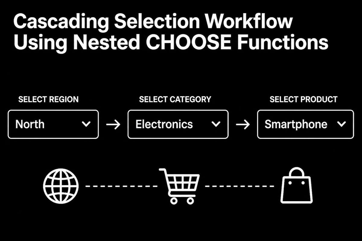
Building Cascading Selection Systems
The choose function excel enables sophisticated cascading menus where one selection determines available options for subsequent choices. By nesting CHOOSE functions or combining them with data validation, you create interactive selection systems.
For example, selecting a region might determine which product list appears next, then selecting a product determines available size options. While this requires careful planning, it creates user-friendly interfaces without VBA programming.
Replacing Complex Nested IF Statements
One of the most valuable applications involves converting nested IF statements into cleaner CHOOSE formulas. A formula like =IF(A1=1,"Red",IF(A1=2,"Blue",IF(A1=3,"Green",IF(A1=4,"Yellow","Other")))) becomes simply =CHOOSE(A1,"Red","Blue","Green","Yellow").
This transformation offers multiple benefits:
- Reduces formula length by 50-70% in most cases
- Eliminates nested parentheses that cause editing errors
- Improves formula auditing and debugging
- Decreases calculation overhead slightly
The MakeUseOf guide demonstrates several real-world scenarios where CHOOSE significantly simplifies complex conditional logic.
Comparing Choose Function Excel to Alternatives
Understanding when to use the choose function excel versus alternative approaches helps you select the optimal solution for each scenario. Different functions excel in different situations.
CHOOSE vs. VLOOKUP/XLOOKUP
VLOOKUP and XLOOKUP search for values within tables, while CHOOSE selects based on position. CHOOSE works best when you know the exact position and have a limited set of predetermined values. VLOOKUP excels when searching large tables for matching criteria.
| Feature | CHOOSE | VLOOKUP/XLOOKUP |
|---|---|---|
| Best for | Fixed set of values | Large lookup tables |
| Speed | Faster for small sets | Better for large datasets |
| Flexibility | Limited to 254 values | Unlimited rows |
| Maintenance | Easy inline editing | Requires table management |
| Dynamic ranges | Not supported | Fully supported |
For projects requiring professional Excel consulting, we evaluate which lookup method best balances performance and maintainability for your specific use case.
CHOOSE vs. IFS Function
Excel's IFS function, introduced in Excel 2016, provides another alternative to nested IF statements. IFS evaluates multiple conditions sequentially, while CHOOSE requires a numeric index.
CHOOSE proves more efficient when you have a numeric selector, while IFS works better with complex logical conditions that don't translate cleanly to position numbers. For simple numeric mapping, CHOOSE typically performs faster and produces more concise formulas.
CHOOSE vs. SWITCH Function
The SWITCH function, available in Excel 2016 and later, offers functionality similar to CHOOSE but with more flexibility. SWITCH matches expressions to values, allowing text-based matching rather than requiring numeric indices.
=SWITCH(A1, "Red", 1, "Blue", 2, "Green", 3) accomplishes what would require combining MATCH and CHOOSE. However, CHOOSE remains useful when working with sequential numeric codes or when compatibility with older Excel versions matters.
As detailed in ExcelJet’s function comparison, each function has optimal use cases, and experienced users leverage the strengths of each approach.
Real-World Implementation Scenarios
Applying the choose function excel to actual business problems demonstrates its practical value beyond theoretical examples. These scenarios reflect common challenges encountered in professional spreadsheet work.
Sales Commission Calculator
A sales organization with four product lines assigns different commission rates to each. Rather than maintaining a lookup table, the commission calculator uses CHOOSE to select the appropriate rate based on the product code.
The formula =sales_amount * CHOOSE(product_code, 0.05, 0.08, 0.10, 0.12) multiplies the sale amount by the commission rate. Product code 1 receives 5%, code 2 receives 8%, and so forth. This approach embeds business logic directly into the calculation, reducing dependencies on external reference data.
When sales managers need to adjust rates, they can quickly update the formula values rather than maintaining separate rate tables. This simplification reduces potential errors from mismatched references or outdated lookup data.
Project Status Dashboard
Project managers tracking multiple initiatives often need to display status indicators based on completion percentages. The choose function excel enables automatic status assignment without complex conditional formatting rules.
Using =CHOOSE(MIN(5,INT(completion_percentage/20)+1), "Not Started", "Planning", "In Progress", "Nearly Complete", "Finished") automatically assigns status text based on completion percentage ranges. 0-19% shows "Not Started," 20-39% shows "Planning," and so on through 80-100% showing "Finished."
The MIN function ensures the index never exceeds 5, preventing errors if completion_percentage somehow exceeds 100%. This robust approach prevents common edge case failures.
Expense Category Reporting
Finance departments categorizing expenses often receive transaction codes from accounting systems. Converting these codes to readable category names for management reports becomes straightforward with CHOOSE.
A formula like =CHOOSE(VLOOKUP(transaction_id, code_table, 2, FALSE), "Travel", "Meals", "Supplies", "Equipment", "Services", "Other") first looks up the category code, then uses CHOOSE to return the descriptive text. This two-step process maintains data integrity while improving report readability.
For organizations seeking Excel business automation, these combined techniques create powerful self-updating reports that reduce manual data manipulation.
Seasonal Adjustment Factors
Retail and hospitality businesses applying seasonal adjustment factors to forecasts benefit from CHOOSE's ability to select month-specific multipliers. The formula =base_forecast * CHOOSE(MONTH(forecast_date), 0.85, 0.90, 1.05, 1.10, 1.15, 1.20, 1.15, 1.10, 0.95, 0.90, 1.05, 1.30) adjusts the base forecast by month-specific factors.
December (month 12) receives a 1.30 multiplier for holiday shopping, while January (month 1) applies 0.85 to account for post-holiday slowdowns. This single formula replaces twelve separate conditional calculations, significantly reducing formula complexity and maintenance burden.
Integration with Modern Excel Features
The choose function excel continues to evolve as Microsoft enhances Excel with new capabilities. Understanding how CHOOSE works with modern features ensures you leverage the full power of current Excel versions.
Dynamic Arrays and Spilling
In Excel 365 and Excel 2021, dynamic array formulas automatically spill results to adjacent cells. CHOOSE can return arrays that spill, creating powerful single-formula reports.
The formula =CHOOSE(selector, sales_array, cost_array, profit_array) returns an entire array based on the selector value. When selector equals 2, the entire cost_array spills into the spreadsheet, eliminating the need to copy formulas down columns.
This capability transforms dashboard creation by enabling single-cell formulas that populate entire report sections based on user selections or calculated criteria.
LET Function for Readability
The LET function, introduced in Excel 365, assigns names to calculation results for use within formulas. Combining LET with CHOOSE improves readability in complex formulas.
=LET(
    quarter, CHOOSE(ROUNDUP(MONTH(A2)/3,0), "Q1", "Q2", "Q3", "Q4"),
    sales, SUM(sales_range),
    quarter & ": $" & TEXT(sales, "#,##0")
)
This approach calculates the quarter using CHOOSE, assigns it to the variable "quarter," then uses that variable in the final text assembly. Breaking complex formulas into named components dramatically improves maintainability.
FILTER and SORT Compatibility
Modern filtering and sorting functions work seamlessly with CHOOSE results. You can filter or sort data based on CHOOSE output, enabling sophisticated data presentation without pivot tables.
The formula =FILTER(data_range, CHOOSE(status_column, condition1, condition2, condition3)) filters the data range based on dynamically selected conditions. This creates interactive filtered views controlled by simple dropdown selections.
Resources like Computer Gaga’s tutorial demonstrate how these modern combinations create powerful analytical tools with minimal complexity.
Power Query Integration
When building data models that combine Excel formulas with Power Query transformations, CHOOSE formulas in source tables properly refresh when Power Query reloads data. This reliability makes CHOOSE valuable for pre-transformation calculations that feed into Power Query workflows.
However, consider performing categorical mappings within Power Query itself when dealing with large datasets, as M language transformations often outperform worksheet formulas for high-volume operations.
Mastering the choose function excel provides a powerful tool for simplifying data selection tasks, replacing complex nested formulas, and creating more maintainable spreadsheets. Whether you're mapping numeric codes to descriptive text, building dynamic calculators, or designing interactive dashboards, CHOOSE offers an elegant solution that balances simplicity with capability. If you're struggling with complex formulas, need help optimizing your spreadsheet performance, or want personalized training on Excel functions like CHOOSE, The Analytics Doctor provides expert guidance tailored to your specific needs. From diagnosing formula errors to building automated reporting solutions, you'll receive practical support that transforms how you work with data.