
Imagine unlocking a new level of efficiency in Excel, where finding the right data is quick, accurate, and stress-free. In 2026, mastering how to use xlookup is the key to transforming your data management skills.
This essential guide will show you how to use xlookup, breaking down its features and advantages over older lookup functions. You will discover step-by-step instructions, advanced techniques, troubleshooting tips, and real-world business applications.
Get ready to streamline your workflow, solve data challenges with confidence, and take full control of your spreadsheets using Excel’s most powerful lookup tool.
Understanding XLOOKUP: What It Is and Why It Matters in 2026
Imagine being able to search any direction in your data and find exactly what you need in seconds. That is the promise of XLOOKUP, Excel’s most versatile lookup function, now a standard feature in 2026. If you have ever wondered how to use xlookup to eliminate the headaches of traditional lookups, this is where your journey begins.

What is XLOOKUP?
XLOOKUP is a breakthrough Excel function developed for Microsoft 365 and now available across Excel 2021 and Excel for web. It lets you search for a value in a range or array and return the corresponding value from another range, no matter where that data sits in your table. Unlike its predecessors, XLOOKUP works left to right, right to left, or even vertically and horizontally with equal ease. If you have been seeking how to use xlookup to streamline your daily data tasks, you are in the right place.
Supported platforms include:
- Microsoft 365 (Windows/Mac)
- Excel 2021 and later
- Excel for web
Why XLOOKUP Matters in 2026
Before XLOOKUP, Excel users relied on VLOOKUP and HLOOKUP, which forced you to organize data in rigid columns or rows. These older functions could not search to the left, required static column numbers, and were prone to errors. XLOOKUP solves these issues with a simpler syntax, dynamic ranges, and robust error handling. Learning how to use xlookup means fewer formula headaches, faster reporting, and cleaner dashboards.
Key benefits include:
- No left/right lookup restrictions: Search any direction.
- Simplified syntax: Fewer arguments and no need to count columns.
- Improved error handling: Customizable error messages.
- Flexible matching options: Exact, approximate, or wildcard matches.
For a detailed breakdown of its arguments and capabilities, see the XLOOKUP function – Microsoft Support page.
Comparing XLOOKUP and VLOOKUP: A Simple Example
Let’s see how to use xlookup with a practical example. Imagine you have a table with Product IDs in column A and Product Names in column B.
With VLOOKUP:
=VLOOKUP("P100", A2:B100, 2, FALSE)
- Must search left to right.
- Requires column number.
With XLOOKUP:
=XLOOKUP("P100", A2:A100, B2:B100)
- Searches any direction.
- No column number needed.
This flexibility allows you to restructure your data without constantly adjusting your formulas. XLOOKUP also reduces the risk of errors when ranges change or new columns are added.
The Rise of XLOOKUP: Essential for Modern Data Work
Since its introduction in 2020, XLOOKUP has rapidly replaced VLOOKUP, HLOOKUP, and even many INDEX/MATCH setups. Today, knowing how to use xlookup is considered a must-have skill for analysts, managers, and anyone who works with data. Its adoption has been swift, driven by the need for more flexible, reliable, and efficient data analysis tools.
Businesses now rely on XLOOKUP for everything from financial modeling to real-time dashboards and advanced business intelligence. As Excel continues to evolve, mastering XLOOKUP is one of the smartest investments you can make in your professional toolkit.
Anatomy of the XLOOKUP Function: Syntax and Arguments Explained
Mastering how to use xlookup begins with understanding its flexible syntax and arguments. XLOOKUP is designed to be intuitive, replacing older lookup functions with a streamlined structure that adapts to a wide variety of Excel scenarios.
XLOOKUP Syntax: The Complete Structure
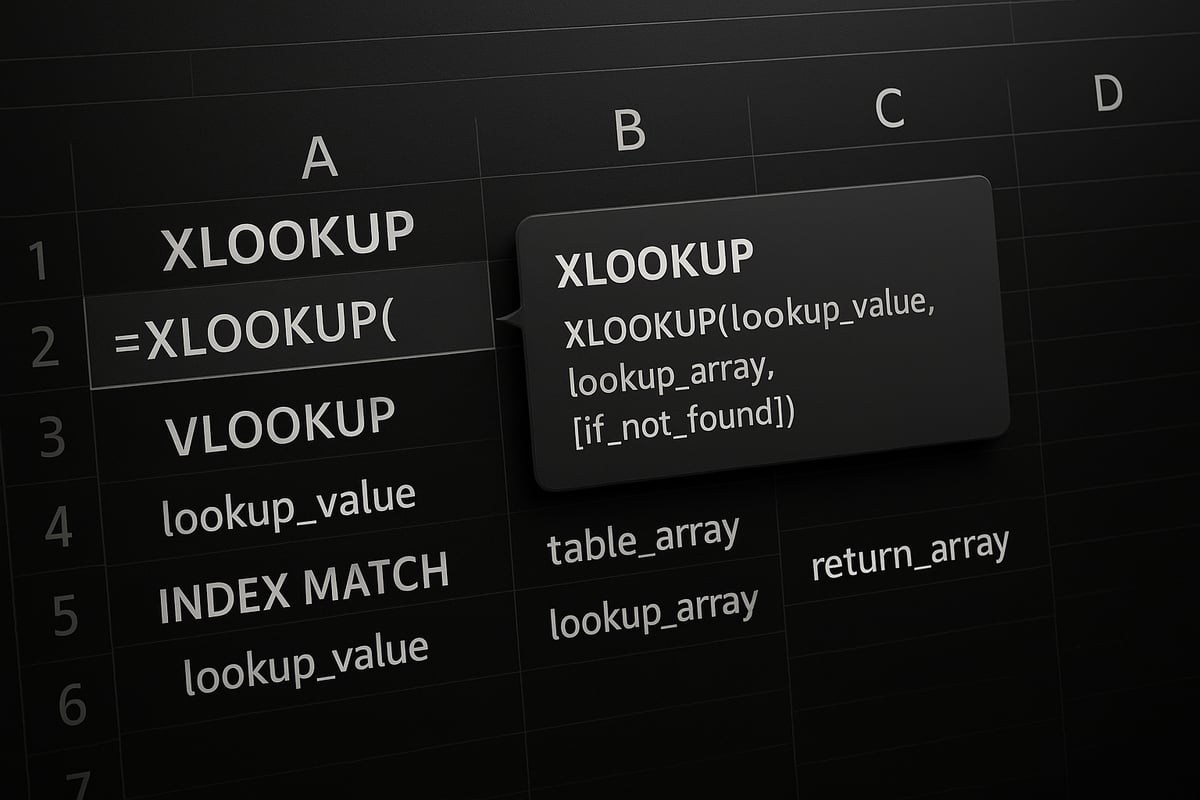
The full syntax for XLOOKUP is:
=XLOOKUP(lookup_value, lookup_array, return_array, [if_not_found], [match_mode], [search_mode])
Here is what each argument means when you learn how to use xlookup:
- lookup_value: The item you want to find.
- lookup_array: The range or array where Excel searches for your lookup_value.
- return_array: The range or array from which to return a result.
Optional arguments give you more control:
- [if_not_found]: Display a custom message or value if nothing is found.
- [match_mode]: Set to 0 for exact match, -1 or 1 for next smaller/larger, 2 for wildcards.
- [search_mode]: Choose search direction: 1 for first-to-last, -1 for last-to-first, 2 or -2 for binary search.
Practical Examples for Each Argument
Using how to use xlookup in practice, consider this annotated formula:
=XLOOKUP("P100", A2:A100, B2:B100, "Not found", 0, 1)
- This searches for "P100" in column A, returns the matching value from column B, displays "Not found" if missing, forces an exact match, and searches from first to last.
If you omit optional arguments, XLOOKUP defaults to exact match (0), and first-to-last search (1). If no match exists and no [if_not_found] is set, you’ll see a #N/A error.
Error Handling with XLOOKUP
With how to use xlookup, error handling is much improved. Instead of cryptic errors, you can set friendly messages:
=XLOOKUP("Jane", A2:A100, B2:B100, "No match found")
This approach helps users avoid confusion and streamlines troubleshooting.
XLOOKUP vs. VLOOKUP/HLOOKUP/INDEX-MATCH: Argument Comparison
Below is a summary table showing how argument structures compare:
| Function | Lookup Value | Lookup Array | Return Array | Custom Error | Match Mode | Search Mode |
|---|---|---|---|---|---|---|
| XLOOKUP | Yes | Yes | Yes | Yes | Yes | Yes |
| VLOOKUP | Yes | Yes | No | No | Yes | No |
| HLOOKUP | Yes | Yes | No | No | Yes | No |
| INDEX/MATCH | Yes | Yes | Yes | No | Yes | No |
XLOOKUP’s flexible syntax and rich options have made it the go-to lookup tool for Excel users, as explained in Announcing XLOOKUP, successor to the iconic VLOOKUP.
Real-World Example: Employee Directory Lookup
Suppose you have an employee list and want to find an email by name. Using how to use xlookup, the formula is:
=XLOOKUP("Alice", A2:A100, C2:C100, "Employee not found")
If "Alice" does not exist, the formula returns "Employee not found" instead of an error.
Conclusion
Understanding the anatomy of XLOOKUP is essential for anyone who wants to know how to use xlookup efficiently in 2026. By mastering its arguments and leveraging optional settings, you can replace outdated lookup formulas and solve real-world data challenges with confidence.
Step-by-Step Guide: How To Use XLOOKUP in Excel
Mastering how to use xlookup in Excel begins with understanding your data and building confidence with the function's flexible structure. This step-by-step guide will help you unlock XLOOKUP’s potential, whether you are new to the feature or looking to refine your approach for 2026.

Preparing Your Data for XLOOKUP
Before you learn how to use xlookup, focus on your data’s structure. Clean, organized data is essential for reliable results. XLOOKUP is more forgiving than older lookup tools, but it still performs best when your tables are tidy.
Unlike VLOOKUP, there’s no need to rearrange columns. XLOOKUP can search left, right, up, or down. Start by removing duplicates and ensuring there are no blank cells in your lookup arrays. This step minimizes errors and speeds up your workflow.
For example, if you are setting up an employee or sales table, check that each entry is unique and each column uses consistent data types. Numbers and text should not be mixed within the same field. When you know how to use xlookup with clean data, you gain accuracy and save time.
Tips for large datasets:
- Use filters to spot inconsistencies
- Convert data ranges to Excel Tables for easier management
- Run a quick check for extra spaces or non-printing characters
Proper data preparation builds a solid foundation for all future XLOOKUP operations.
Building a Basic XLOOKUP Formula
Now, let’s explore how to use xlookup for a simple lookup. Suppose you have a table with Product IDs in column A and Product Names in column B. Your goal is to find the name for a specific ID.
Follow these steps:
- Identify your
lookup_value(e.g., "P100"). - Define your
lookup_array(A2:A100). - Choose your
return_array(B2:B100).
Enter the formula:
=XLOOKUP("P100", A2:A100, B2:B100)
This returns the product name for "P100". Common mistakes when learning how to use xlookup include mismatched ranges and inconsistent data types. Always make sure your lookup and return arrays are the same size.
If your formula isn’t working, try Excel’s Evaluate Formula feature to step through the calculation. This tool helps pinpoint where things might be going wrong.
Quick troubleshooting tips:
- Double-check range selections
- Confirm data type consistency
- Review for hidden characters
Getting comfortable with these basics ensures you know how to use xlookup with confidence.
Using Optional Arguments for Customization
To truly master how to use xlookup, you need to leverage its optional arguments. These options let you customize what happens when a value isn't found, set match types, and control search direction.
if_not_found: Displays a custom message if no match is found.match_mode: Choose between exact match (0), next smaller (-1), next larger (1), or wildcard (2).search_mode: Select search direction, like first-to-last (1) or last-to-first (-1).
Example formula:
=XLOOKUP("Jane", A2:A100, B2:B100, "No match", 0, -1)
This searches from last to first for "Jane" and returns "No match" if she isn't found. When exploring how to use xlookup with optional settings, remember to match the options to your specific scenario.
Avoid these pitfalls:
- Forgetting to adjust match_mode for approximate matches
- Using wildcards without setting match_mode to 2
- Mismatched range sizes when adding optional arguments
Mastering these customizations takes your XLOOKUP skills to the next level.
Practical Example: Multi-criteria Lookup with XLOOKUP
Sometimes you need to know how to use xlookup for more complex lookups, like combining first and last names to find an employee’s ID. XLOOKUP can handle multi-criteria searches by concatenating values.
Suppose you have first names in A2:A100, last names in B2:B100, and IDs in E2:E100. To search for a unique combination, use:
=XLOOKUP(A2&B2, C2:C100&D2:D100, E2:E100)
This approach is helpful when you have duplicate names in your dataset. Be aware that concatenated keys must match exactly, including spaces and case sensitivity.
Limitations:
- Does not handle partial matches unless combined with wildcards
- May require helper columns for clarity
Workarounds include creating a new column with the combined key for easier maintenance.
Troubleshooting XLOOKUP Errors
No matter how well you know how to use xlookup, errors can still occur. The most common is the #N/A error, often caused by missing data or mismatched ranges.
Other issues include:
- Range size mismatches between lookup and return arrays
- Data type mismatches, such as numbers stored as text
- Blank results when the value does not exist
To resolve these, check your source data, use the if_not_found argument for user-friendly messages, and audit formulas with Excel’s built-in tools. For advanced troubleshooting, you can reference this guide on Troubleshooting Excel formulas and errors, which covers deeper diagnostic steps.
Remember to use the F9 key to evaluate parts of your formula and Excel’s formula auditing features for a systematic review. With these strategies, you can resolve most XLOOKUP issues quickly and efficiently.
Advanced XLOOKUP Techniques for Power Users
Unlocking the full potential of XLOOKUP elevates your Excel skills from competent to expert. As you master how to use xlookup in complex scenarios, you will discover its true versatility for business intelligence and data analytics. This section guides you through advanced techniques, ensuring you get the most out of XLOOKUP in 2026.

Approximate Matches, Wildcards, and Range Lookups
Learning how to use xlookup for approximate matches, wildcards, and range lookups opens up new possibilities for data analysis. The match_mode argument lets you control whether XLOOKUP finds exact or closest matches. For example, to assign commission rates based on sales thresholds, set match_mode to -1 (next smaller) or 1 (next larger):
=XLOOKUP(50000, A2:A10, B2:B10, "No rate", -1)
Wildcards are essential when you need partial text matches. Use match_mode 2 to enable wildcards like * (any sequence) or ? (single character):
=XLOOKUP("Pro*", A2:A100, B2:B100, "Not found", 2)
For sorted data, binary search (search_mode 2 or -2) significantly boosts performance. This is crucial when handling large datasets, as XLOOKUP can process lookups much faster. If you are deciding between XLOOKUP and INDEX/MATCH for speed and flexibility in these scenarios, consider this in-depth comparison between XLOOKUP and INDEX MATCH for further insights.
Mastering these options is key to understanding how to use xlookup for advanced lookups that streamline reporting workflows.
Bi-directional and Reverse Lookups
One of the biggest advantages of learning how to use xlookup is its ability to perform lookups in any direction. Unlike VLOOKUP, which only searches to the right, XLOOKUP retrieves data left, right, up, or down. For example, if you need to find a product ID given its name and the name column is to the right of the ID, use:
=XLOOKUP("Widget", B2:B100, A2:A100)
Reverse searches are invaluable when you want the last occurrence of a value, such as finding the most recent transaction for a customer. Set search_mode to -1:
=XLOOKUP("John Doe", A2:A100, B2:B100, , 0, -1)
This approach solves common business challenges, like retrieving the latest status or historical data. Knowing how to use xlookup for reverse and bi-directional lookups gives you flexibility that legacy functions lack.
Nested XLOOKUPs and Dynamic Arrays
As you advance in how to use xlookup, you will encounter scenarios needing multi-level or compound lookups. Nesting XLOOKUP allows you to fetch data based on the result of another lookup. For example, to find a manager after looking up a region:
=XLOOKUP(XLOOKUP("Jane", A2:A100, B2:B100), D2:D100, E2:E100)
Dynamic arrays let you spill results for multiple lookups at once. For instance, retrieving product prices for a list of IDs:
=XLOOKUP(A2:A10, C2:C100, D2:D100)
Excel 2026 fully supports dynamic arrays, so how to use xlookup in this context is now seamless. You can aggregate, filter, or analyze multiple results without complex formulas. This transforms how analysts handle large data extractions and reporting.
Integrating XLOOKUP with Other Excel Functions
For true power, combine how to use xlookup with other Excel functions. Pair XLOOKUP with IF for conditional lookups, such as:
=IF(XLOOKUP("Sally", A2:A100, B2:B100, "")="Manager", "Approve", "Review")
Use XLOOKUP inside SUM or FILTER to build dynamic dashboards. For example, summing sales by region after a lookup:
=SUMIF(D2:D100, XLOOKUP("East", A2:A100, C2:C100), E2:E100)
These integrations automate monthly updates and streamline reporting. Mastering how to use xlookup in combination with other functions amplifies your efficiency and reduces manual errors in business workflows.
Real-World Applications and Business Scenarios for XLOOKUP
XLOOKUP has rapidly become a cornerstone for data-driven teams in every industry. Mastering how to use xlookup empowers professionals to solve daily business challenges with speed and accuracy. Let’s explore practical scenarios where xlookup shines and see why it’s now a must-have skill for 2026.

HR, Sales, and Finance Applications
In human resources, knowing how to use xlookup streamlines employee directory management, benefits lookup, and attendance tracking. You can instantly retrieve contact details, department data, or benefits eligibility from large tables, saving valuable time.
Sales teams rely on xlookup for quick price list lookups, commission calculations, and comprehensive sales reporting. When product IDs or customer names change, xlookup adapts without the rigid limitations of old lookup functions.
Finance departments benefit from xlookup’s versatility in budget reconciliation, account mapping, and variance analysis. By pulling data from multiple sources, finance professionals can ensure reports stay accurate and up-to-date.
Operations, Education, and Analytics
Operational teams use xlookup for inventory tracking, supplier lookups, and order fulfillment. It enables real-time matching of stock numbers with supplier information, reducing delays and errors.
Educators and administrators appreciate how to use xlookup for grade lookups, student records, and course assignments. Managing large student databases becomes effortless, especially when dealing with duplicate names or complex enrollment data.
Data analysts depend on xlookup for merging datasets, cleaning records, and building dynamic reports. Ensuring data integrity is crucial, so applying Excel data validation rules and checks helps keep lookup results reliable and actionable.
Example: Matching Sales Transactions
Imagine a scenario where you need to match thousands of sales transactions with corresponding customer data. By learning how to use xlookup, you can link transaction IDs to customer names, addresses, or purchase history in just seconds. This process eliminates manual cross-referencing and reduces the risk of mismatched or missing data.
A typical formula might look like:
=XLOOKUP(A2, CustomerIDs, CustomerNames, "Not Found")
This instantly returns the customer name for each transaction, even in massive datasets.
Streamlining Processes: XLOOKUP vs. Legacy Methods
Legacy lookup functions, like VLOOKUP and HLOOKUP, often required cumbersome workarounds and static column indices. They couldn’t search to the left or above, which limited their usefulness. Now, understanding how to use xlookup means you can search in any direction, use custom error messages, and handle dynamic data ranges with ease.
Here’s a quick comparison:
| Feature | VLOOKUP/HLOOKUP | XLOOKUP |
|---|---|---|
| Direction | Right/Below only | Any direction |
| Error Handling | Limited | Customizable |
| Syntax | Complex | Simple |
| Flexibility | Low | High |
Adopting xlookup not only streamlines workflows but also reduces manual errors significantly.
Case Study: Time Savings and Error Reduction
A mid-sized business recently transitioned to xlookup for their monthly sales and payroll processes. Before, reconciling sales data with payroll records took several hours and was prone to mistakes. After training the team on how to use xlookup, the process now takes minutes, and error rates have dropped dramatically.
Implementing systematic checks, like those described in Reduce spreadsheet errors in Excel, further enhanced data accuracy and team confidence.
Tips for Scaling XLOOKUP in the Enterprise
As your organization grows, scaling xlookup usage requires a few best practices:
- Use named ranges for better formula clarity.
- Document lookup formulas for team transparency.
- Regularly audit data sources to prevent mismatches.
- Train staff on how to use xlookup in various scenarios.
- Automate recurring tasks with templates and macros.
By embedding these habits, you ensure xlookup remains a powerful tool for operational excellence and strategic decision-making.
Expert Tips, Common Pitfalls, and Best Practices for XLOOKUP Success
Mastering how to use xlookup is about more than just memorizing syntax. Applying expert strategies and knowing common traps can transform your Excel experience, making your work faster, cleaner, and more reliable.
Best Practices for Reliable XLOOKUP Formulas
To excel at how to use xlookup, start by structuring your data tables with clear headers and consistent data types. Use named ranges for lookup and return arrays to make formulas easier to read and maintain. Document your formulas with cell comments or a separate sheet, so others can quickly understand your approach.
Keep your source data clean. Remove duplicates, ensure no hidden blanks, and standardize text or number formats. This avoids mismatches that can break your lookups. When using XLOOKUP across large datasets, double-check that your lookup and return arrays are the same size. This is a common oversight.
If you are migrating from older functions, familiarize yourself with the differences. For a deeper comparison, see XLOOKUP vs. VLOOKUP vs. INDEX/MATCH: Which to Use in 2025?. Understanding these distinctions will help you avoid legacy pitfalls and fully leverage the flexibility of how to use xlookup.
Avoiding Common Pitfalls and Errors
Even seasoned users can trip up on subtle issues. One frequent problem is mismatched data types: numbers stored as text or vice versa. Always check that your lookup values and arrays use the same format. Use Excel’s ISTEXT and ISNUMBER functions to diagnose problems.
Another pitfall is range size mismatches. Both lookup_array and return_array must have the same number of rows or columns. If not, XLOOKUP will return an error. Watch for blank cells, which can cause unexpected results or missed matches.
To handle missing data gracefully, use the if_not_found argument to display custom messages like "No result found." This makes your models user-friendly and robust. Also, when troubleshooting, use Excel’s Evaluate Formula tool or press F9 to inspect calculation steps. These habits are essential for anyone mastering how to use xlookup.
Performance, Security, and Collaboration
When working with large workbooks, efficiency matters. Limit the size of ranges used in XLOOKUP to only what is necessary. Avoid volatile functions in combination with XLOOKUP, as they can slow down recalculation.
For sensitive data, protect your lookup ranges with worksheet protection and restrict access as needed. Be mindful when sharing files with others, especially in collaborative settings. Use named ranges and document formula logic to make it easier for teams to understand and update your work.
If you often compare spreadsheets or audit data, consider leveraging specialized guides like Compare spreadsheets with formulas and tools. Integrating such techniques with how to use xlookup can significantly streamline your review process.
Upgrading, Resources, and Optimization Checklist
Transitioning from VLOOKUP or HLOOKUP to XLOOKUP is a smart move for 2026. Start by identifying all legacy lookups and replacing them with XLOOKUP. Test each formula for accuracy and document any changes. Stay informed about new Excel features by following Microsoft’s official documentation and reputable Excel blogs.
For ongoing support, join Excel communities and forums. These resources are invaluable for troubleshooting and learning advanced techniques. To ensure you always optimize how to use xlookup, keep this quick checklist handy:
**XLOOKUP Optimization Checklist**
- Use named ranges for clarity
- Match data types between lookup and return arrays
- Remove blanks and duplicates
- Test formulas with Evaluate Formula
- Leverage `if_not_found` for user-friendly errors
- Document formulas and updates
By following these steps and staying engaged with Excel’s evolving ecosystem, you will remain at the forefront of how to use xlookup effectively.

