How to Build an Excel Dependent Drop Down List: Step‑by‑Step Guide

Ever stared at a spreadsheet that feels like a maze, wondering why everyone keeps picking the wrong options?

You’re not alone. Most of us have spent minutes—sometimes hours—cleaning up mismatched entries that could have been prevented with a smarter setup.

Enter the excel dependent drop down list: a simple trick that lets one choice automatically filter the next, keeping data tidy without extra effort.

Imagine you have a list of regions, and once you pick “Europe,” the city dropdown instantly shows only Paris, Berlin, Madrid, and so on. No more scrolling through a thousand rows looking for the right match.

Sounds like magic? It’s really just a couple of formulas and the built‑in Data Validation feature working together.

In practice, this approach saves time, reduces errors, and makes your workbook feel almost conversational—you select, and the sheet responds.

But why bother? Think about the last time a sales report got delayed because someone entered “NY” under a “Country” column. A dependent list would have stopped that mistake at the source.

And it’s not just for sales. HR teams use it to lock down job titles under departments, finance folks to tie expense categories to sub‑categories, anyone who wants clean, reliable data.

What’s even better is that you don’t need a VBA wizard or a pricey add‑on. Excel’s native tools handle it, and once you set it up, the list works across the whole workbook.

So, if you’ve ever felt frustrated watching a colleague type “Apple” into a “Fruit Type” column that only accepts “Citrus,” you know the pain point this solves.

Ready to turn that frustration into a smooth, error‑free experience? We’ll walk through the core steps, share a few pro tips, and show how you can apply the technique to any project.

Grab a coffee, fire up Excel, and let’s make your data entry feel as natural as a conversation.

TL;DR

An excel dependent drop down list lets you pick a main option and instantly shows only relevant choices for the next field, cutting errors and saving minutes of data‑cleaning.

Set it up with a few named ranges and INDIRECT—no VBA required—and you’ll turn messy sheets into smooth, conversation‑like entry points.

Ever opened a fresh sheet and felt the panic of “where do I even start?” You’re not alone. The first step in any excel dependent drop down list is to give it something solid to lean on – a tidy source table.

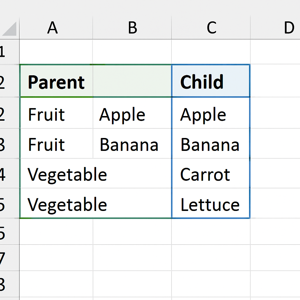
Grab a new worksheet and call it Lists. In column A, type your main categories – think Region, Department, or Product Line. Below each header, list every option you want to appear in the first drop‑down.

Next to each parent column, create a matching child column. If A holds regions, B could hold the cities that belong to each region, C the offices, and so on. Keep the layout simple: one column per parent, one column per child.

Now, a little gotcha: Excel won’t like spaces in named ranges. The Microsoft community points out that spaces are automatically turned into underscores, and that can break the INDIRECT formula if you’re not careful Microsoft’s guidance on creating dependent drop‑down lists. So rename Sub Category as Sub_Category or just drop the space altogether.

With the raw data in place, turn each column into a named range. Select the whole column of regions (excluding the header), click the Name Box left of the formula bar, and type Region. Do the same for every child list, using the exact text you’ll later reference in the INDIRECT formula – remember those underscores.

Tip: if you expect the list to grow, define the name as a dynamic range. A quick =OFFSET(Region,0,0,COUNTA(Region),1) will automatically expand as you add new entries.

Because you’ll be pulling these lists from a different sheet than your data entry area, it’s best practice to keep the source sheet hidden or very far to the right. The Power Apps documentation recommends separating source data from the user‑facing sheet to avoid accidental edits best practice for separating source data. In Excel, you can simply right‑click the Lists tab and choose “Hide”.

Once your names are defined, you can test them. Click any empty cell, type =Region and hit Enter – you should see the array of regions spill out. If you get a #NAME? error, double‑check the name spelling and that there are no stray spaces.

Now that the foundation is solid, the dependent drop‑downs will have a reliable source to query. The rest of the setup – adding data validation and the INDIRECT magic – will be painless because Excel knows exactly where to look.

Need a visual refresher? Watch the short walkthrough below; it walks through creating the source list, naming ranges, and hiding the sheet – all in under five minutes.

Take a breath. You’ve just turned a chaotic pile of text into a structured data model. When you move on to step two, the dependent drop‑down will instantly pull the right choices, and you’ll wonder how you ever lived without it.

Alright, the source table is ready and named. Now we need the first drop‑down that your users will actually click.

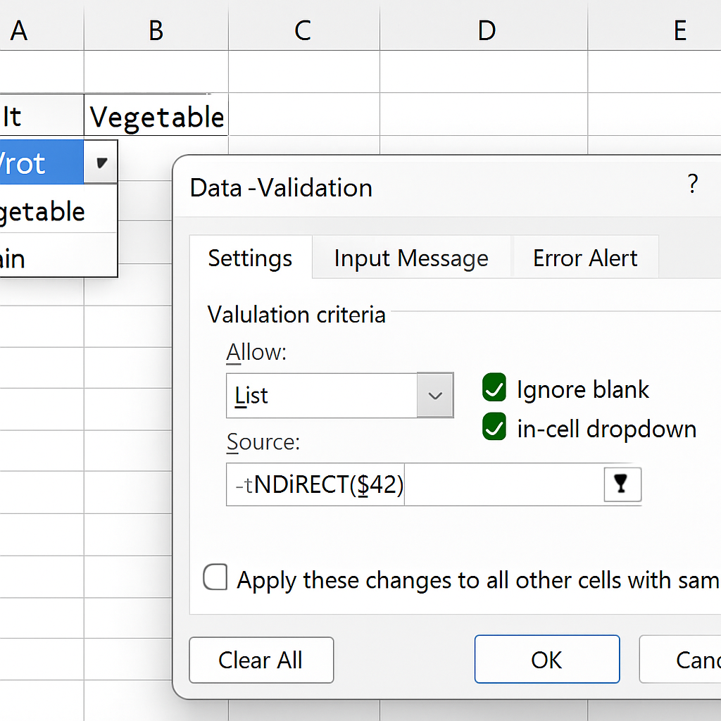
First, pick the cell (or column) where you want the primary list to appear – maybe column A on your data‑entry sheet. Click it, then head to the Data tab and hit Data Validation. In the dialog, set “Allow” to “List”.

In the “Source” box, type the name you gave the parent range, for example =Region. Excel will pull every region you entered earlier and display them as choices.

Quick sanity check

After you hit OK, click the arrow that appears. Do you see all your regions? If you only get a handful, double‑check the named range – a stray space or hidden character can break the list.

That’s actually a common hiccup. In a Microsoft community thread, a user reported three items in the first‑level list that simply didn’t react, and the fix was to hunt down hidden characters in the source data according to the community discussion.

Tip: Use a table for dynamic growth

If you expect the list to expand, convert your source column to an Excel Table (Ctrl+T). Tables automatically adjust their size, and any named range that references the table column will grow with it. No need to edit the validation source every time you add a new region.

And because tables give each column a structured reference, you could even write the source as =Lists[Region] instead of a separate name – whatever feels cleaner for you.

Locking down the list

To keep users from typing free‑form text, make sure the “In‑cell dropdown” box stays checked. You can also tick “Ignore blank” if you want to allow empty cells before a selection is made.

One more safeguard: go to the “Error Alert” tab and customize the message. Something friendly like “Please pick a region from the list – we’ll handle the rest” feels more human than a generic #VALUE! error.

Now you’ve got a solid primary drop‑down. The next step will be to make the secondary list listen to whatever the user picks here, but before we get there, let’s make sure this list behaves like a pro.

Testing like a detective

Pick a few cells, change the selection, and watch the list update. If you notice any duplicate entries, go back to the source column and remove the repeats – duplicates will show up in the dropdown too.

Also, remember that named ranges are case‑insensitive, but they can’t contain spaces. If you ever named a range “North America”, Excel silently changed it to “North_America”. If your validation still points to the old name, it won’t work.

And if you ever need to troubleshoot, the “Name Manager” (Formulas → Name Manager) shows you exactly what each name points to. It’s a handy place to spot a typo before it drives you crazy.

Final checklist for the primary list

Cell(s) selected for the list.
Data Validation set to “List”.
Source points to the correct named range (e.g., =Region).
In‑cell dropdown enabled.
Custom error alert added.
Source data free of hidden characters or duplicates.

That’s it. You’ve just turned a bland column into a guided, error‑proof selector. When you move on to the dependent drop‑down, Excel will already know which set of values to pull, making the whole process feel almost magical.

Step 3: Define Dependent Lists with Named Ranges

Now that your primary list is solid, it’s time to give Excel the map it needs to pull the right child values. In other words, we’re going to turn each category—like Region, Department, or Product Line—into a named range that the dependent drop‑down can reference.

Why named ranges are the secret sauce

Think of a named range as a friendly nickname for a block of cells. Instead of remembering “B2:B15”, you can call it East_Region and let Excel do the heavy lifting. This not only makes formulas easier to read, it also lets you swap out the source data without breaking the validation.

Because the name is case‑insensitive and lives in the workbook’s name manager, you can reuse it on any sheet—perfect for the “one‑source‑truth” approach we championed earlier.

Step‑by‑step: creating a dependent named range

1. Go to the sheet that houses your source table (we called it Lists). Select the column that holds the child values for a specific parent. For example, if column B contains cities for each region, highlight B2:B20.

2. Click the Name Box (the field left of the formula bar) and type a concise name—no spaces, no special characters. A good pattern is Region_Europe or Dept_Sales. Press Enter.

3. Repeat the process for every parent option. If you have ten regions, you’ll end up with ten named ranges, each pointing at its own list of cities.

If you’re dealing with a growing list, consider a dynamic range. The classic formula =OFFSET(Cities,0,0,COUNTA(Cities),1) expands automatically as you add new rows. A community member on the Microsoft tech forum swears by this trick for horizontal layouts where locations sit side‑by‑side.

Horizontal vs. vertical named ranges

Most tutorials focus on vertical lists, but real‑world data sometimes arrives in a table where each merchant’s locations are laid out across a row. In that case you’ll need a horizontal named range. The OFFSET syntax flips the width and height arguments: =OFFSET(StartCell,0,0,1,COUNTA(StartCell:EndCell)). The community post above shows exactly how to build it.

Once the horizontal range is defined, the dependent validation formula stays the same—Excel’s INDIRECT will resolve the name whether it points to a column or a row.

Hooking the dependent drop‑down to the named range

Select the cell (or column) where the secondary list should appear. Open Data Validation, choose “List”, and in the Source box type =INDIRECT(A2)—assuming A2 holds the primary choice. Excel will look up the text you just typed, find the matching named range, and spill the appropriate values.

If you prefer a more explicit reference, you can concatenate the parent name with an underscore: =INDIRECT($A2 & "_" & $B$1). This is handy when your primary list contains spaces; the underscore replaces them in the named range.

Real‑world example: budgeting merchants

Imagine you run a personal budget and track expenses by merchant and location. Your “Merchant” column lists “McDonald’s”, “Starbucks”, “Walmart”. Each merchant has a horizontal named range called Merchant_McDonalds, Merchant_Starbucks, etc., holding all the stores you’ve visited.

When you pick “Starbucks” in the primary drop‑down, the dependent list instantly shows “Downtown”, “Airport”, “Mall”. No more typing “Starb” and hoping for a match. This exact scenario was described in a YouTube walkthrough that walks through setting up the ranges; the visual makes the concept click.

Watch the quick video for a visual cue: step‑by‑step video guide.

Testing and troubleshooting tips

– After defining each name, type =NameYouCreated in an empty cell. If you see the expected array, the name is correct.

– Use the Name Manager (Formulas → Name Manager) to spot typos. A missing underscore or extra space is a common cause of #REF! errors.

– If the dependent list returns #NAME?, double‑check that the primary cell’s value exactly matches the named range (Excel ignores case but not underscores).

Quick checklist

All child columns have a clean, space‑free named range.
Dynamic ranges use OFFSET or Table references for auto‑growth.
Horizontal lists use the width‑first OFFSET syntax.
Data Validation source points to =INDIRECT(PrimaryCell) (or concatenated version).
Test each name with a simple formula before applying validation.
Document the naming convention somewhere in the workbook (a hidden “Info” sheet works well).

When you’ve checked every box, the dependent drop‑down will behave like a well‑trained assistant—always offering the right options at the right time. And if you ever need a refresher on how to build the whole thing, the 5 Simple Steps to Create Drop Down Lists page walks you through the entire workflow.

Step 4: Apply Data Validation and Test the Dependent List

Alright, we’ve built the named ranges and the primary drop‑down, so it’s time to make the magic happen with Data Validation.

Pick the cells where you want the dependent list to appear – maybe column B on your entry sheet – then head to the Data tab and click Data Validation.

In the dialog set “Allow” to “List” and, in the Source box, drop in the INDIRECT formula that points at the primary cell. A typical entry looks like =INDIRECT($A2) if A2 holds the first choice.

Notice the dollar sign? It locks the column so you can copy the validation down without breaking the reference.

Does that feel a bit like a secret handshake between the two lists? It is – Excel will read the text you picked, look for a matching named range, and spill the right options.

Step‑by‑step checklist

Select the dependent cells and open Data Validation.
Choose “List” as the validation type.
Enter =INDIRECT($A2) (adjust the cell reference to match your primary column).
Make sure “In‑cell dropdown” stays checked.
Optionally set a friendly Error Alert like “Pick a region first, then the city will appear.”
Click OK and drag the corner to apply the rule to the rest of the column.

So, what should you do after you hit OK?

Testing the dependent list

Pick a few rows, choose a value from the primary drop‑down, and watch the second list populate. If you see the expected city names, you’re golden.

If the list stays blank or shows #REF!, open the Name Manager (Formulas → Name Manager) and double‑check that each named range matches the exact text of the primary option – remember, Excel is case‑insensitive but it does care about underscores.

For a quick sanity check, type the named range directly into an empty cell, like =Europe. You should see the array of cities spill out. If you get #NAME?, the name either doesn’t exist or the primary cell’s value isn’t an exact match.

Here’s a handy tip: if your primary list contains spaces (e.g., “North America”), name the range with an underscore (“North_America”) and use a concatenated INDIRECT formula such as =INDIRECT(SUBSTITUTE($A2," ","_")). That tiny tweak saves you from a lot of head‑scratching.

Quick troubleshooting

#REF! – likely a typo or missing named range; fix it in Name Manager.
#NAME? – primary cell value doesn’t match a named range; check underscores and spaces.
List shows duplicate items – clean the source column or make the range dynamic with OFFSET.
Validation won’t copy down – ensure the cell reference in INDIRECT is relative (e.g., $A2, not $A$2).

Ever wonder why other platforms struggle with this? The Airtable community points out that achieving true dependent single‑select behavior often requires convoluted formulas or third‑party tools, highlighting how clean and native Excel’s solution is according to the Airtable discussion.

Once every box in the checklist is ticked, the dependent drop‑down behaves like a well‑trained assistant – it only shows the right choices at the right time, and you’ve avoided a whole class of data‑entry errors.

Give it a spin: pick “Europe” in the primary column and watch “Paris, Berlin, Madrid…” appear instantly. If it works, you’ve just turned a clunky spreadsheet into a conversational data entry experience.

Comparison: INDIRECT vs. Structured Table Formulas for Dependent Lists

We’ve gotten the basic INDIRECT trick working, but now you might be wondering whether there’s a cleaner way once your list starts to grow.

Does the old formula still feel familiar, or is it time to let Excel’s native table engine take the wheel?

Why `INDIRECT` feels familiar

Most of us start with INDIRECT($A2) because it’s quick, it needs no extra setup, and it mirrors the examples we see on countless tutorials.

It works great when you have a handful of named ranges and you don’t expect the source data to change often.

But notice the little quirks: every time you rename a range or add a space, the formula breaks, and you have to chase down #REF! errors.

When structured tables win

Excel tables (Ctrl+T) give you a dynamic range for free. You can reference a column with Lists[Region] and the list expands automatically as you add rows.

Because the table handles sizing, you dodge the blank‑cell problem that often plagues OFFSET or manual named ranges.

In fact, a Stack Overflow discussion points out that using a single named range with OFFSET still pulls blanks, whereas converting the source to a table eliminates them without extra formulas as users have discovered.

Performance and maintenance

With INDIRECT, Excel has to look up a string, resolve it to a range, then fetch the values. That extra lookup can add a tiny lag in very large workbooks.

Tables use structured references, which are cached more efficiently. The result is a snappier drop‑down, especially when you have dozens of dependent columns.

Maintenance is also simpler: rename a table column once, and every validation rule that points to it updates automatically. No hunting through the Name Manager.

Dealing with blanks

If your source list contains occasional empty cells, INDIRECT will happily surface them, leaving an annoying blank option in the drop‑down.

Tables let you filter out blanks directly in the validation source by pointing to the table column – Excel ignores empty rows at the bottom of a table.

And if you still need a pure formula, wrapping the table reference in =FILTER(Lists[City], Lists[City] <> "") gives you a spill range with no blanks, which you then reference with a # sign.

Aspect	INDIRECT	Structured Table
Dynamic range handling	Requires OFFSET or manually updated named ranges	Auto‑expands with table rows
Blank entries	Shows blanks unless extra formula used	Ignores trailing blanks automatically
Maintenance	Rename each named range individually	Rename column once; references follow
Performance	String lookup each time	Structured reference cached, faster
Complexity	Simple for tiny lists, gets messy as list grows	Slight learning curve, but scales cleanly

So, which approach should you pick?

If you’re building a one‑off checklist for a small team, the INDIRECT method gets you up and running in minutes.

But as soon as you anticipate new rows, extra departments, or you just hate chasing #REF! errors, converting the source to a structured table is the smarter, lower‑maintenance route.

Try it out: turn your “Region” column into a table, update the validation source to =Lists[Region], and watch the dependent list stay clean even after you add “South America”.

Either way, the goal stays the same – an excel dependent drop down list that feels like a conversation, not a code battle.

Give it a test run on a real project tomorrow. Pick a few rows, change the primary pick, and see how the dependent list instantly reshapes. You’ll notice the smoother experience and fewer blank entries, proving that the structured‑table route isn’t just theory—it’s a practical time‑saver.

Additional Tips & Troubleshooting Common Issues

You’ve got the primary and dependent drop‑downs wired up, but what happens when something looks a little off?

First, breathe. A blank cell, a #REF! error, or a list that keeps showing the same three items is usually a tiny misstep, not a broken system.

Check the named‑range spelling

Excel is case‑insensitive, but it does care about exact characters. If your primary choice is “North America” and the named range is “North_America”, the space‑to‑underscore mismatch will throw a #REF!.

Open the Name Manager (Formulas → Name Manager) and scan for stray spaces or missing underscores. Fixing a single character often brings the dependent list back to life.

Watch out for hidden characters

Copy‑pasting data from external sources can sneak in non‑printing characters like line breaks or zero‑width spaces. Those invisible gremlins will prevent INDIRECT from finding the right range.

One quick test: select the primary column, go to Find (Ctrl F), click “Options”, and search for “^p” (paragraph break). If you spot anything, replace it with nothing.

Deal with blank entries

Blank rows at the bottom of a named range show up as empty choices in the dependent list. If you’re using a dynamic OFFSET range, make sure the COUNTA part only counts non‑blank cells.

Alternatively, wrap the range in a FILTER that removes blanks, like =FILTER(Region_Europe,Region_Europe<>""), and reference that name in your validation. This keeps the drop‑down tidy without extra cleanup steps.

When INDIRECT feels sluggish

On very large workbooks, the string lookup that INDIRECT performs can introduce a perceptible lag. If you notice the drop‑down pausing after you select a parent value, consider switching to a structured table reference.

Tables cache their column references, so the lookup is faster. Changing the validation source from =INDIRECT($A2) to =Lists[City] (or a FILTER‑wrapped version) often restores snap‑response.

Common #NAME? and #REF! scenarios

Here are the three error types that pop up most often and how to squash them.

#NAME? – The name you typed in the validation formula doesn’t exist. Double‑check the spelling in Name Manager.
#REF! – A named range was deleted or renamed after the validation rule was set. Re‑apply the rule or update the name.
#VALUE! – Usually shows up when the source cell contains an error itself. Clean up the primary list first.

Fixing these three error types usually resolves 90 % of the complaints we hear from users.

Test with a “sandbox” row

Before you roll the list out to the whole team, add a temporary row at the bottom of your entry sheet. Populate the primary drop‑down, watch the dependent list, and note any glitches.

If everything works in that isolated row, you can safely copy the validation down the column. If not, you’ve just isolated the problem without affecting real data.

Video walk‑through for quick debugging

If you prefer a visual guide, the YouTube tutorial walks through each of these pitfalls and shows how to fix them in real time.

Watch the step‑by‑step troubleshooting video for a quick refresher when you hit a snag.

Final quick‑check checklist

Before you call it a day, run through this five‑minute audit.

Named ranges match the exact text of the primary list (underscores for spaces).
No hidden characters or stray line breaks in source columns.
Dynamic ranges use COUNTA or FILTER to exclude blanks.
Consider structured tables if performance feels slow.
Test a sandbox row before copying validation down.
Keep a “Name Manager” snapshot handy for quick audits.

By giving yourself this five‑minute troubleshooting ritual, you’ll keep your excel dependent drop down list humming smoothly, even as the data grows and new team members start using it.

Conclusion

There you have it – you’ve turned a chaotic column into a conversation‑ready excel dependent drop down list. No more hunting for the right city or worrying about a typo slipping through.

Think about the time you spent fixing “NY” in a country field or deleting duplicate entries. With the steps we covered – clean source data, named ranges, and the INDIRECT (or table) validation – those minutes shrink to seconds.

So, what’s the next move? Grab the sheet you just built, add a sandbox row, and watch the dependent list react. If anything feels off, run the quick‑check checklist: named range spelling, hidden characters, blank cells. One tiny tweak usually fixes it.

Remember, the real power isn’t just the formula; it’s the habit of building a five‑minute audit into every new list. That habit keeps your workbook humming as teams grow and data changes.

Finally, treat this as a template. The same approach works for product catalogs, expense categories, or any hierarchy you need to enforce. You’ve got the toolkit – now let your spreadsheets do the heavy lifting.

Next time you set up a new workbook, start with the same clean‑source‑first mindset. You’ll find yourself saving hours and keeping data trustworthy, every single time.

FAQ

What exactly is an excel dependent drop down list and why should I use it?

In plain English, it’s a two‑step dropdown where the second list only shows options that match what you picked in the first. Think of choosing a country first, then seeing just the cities that belong to that country. The magic is that you stop typing nonsense, avoid mismatched data, and speed up entry – all without any VBA or add‑ons.

How do I set up the named ranges without breaking them later?

Start by giving each list a simple, space‑free name – use underscores instead of blanks (e.g., Region_Europe). Define the range on the source sheet, then double‑check it in the Name Manager. If you expect the list to grow, wrap the range in an OFFSET or turn the column into an Excel Table; the name will expand automatically, so you never have to chase #REF! errors again.

My primary dropdown shows the right items, but the dependent one stays blank – what’s wrong?

Most of the time the culprit is a mismatch between the text in the primary cell and the named range. Excel’s INDIRECT is case‑insensitive but it does care about exact characters – spaces, underscores, hidden line‑breaks will all break the link. Open the source column, run a quick Find for ^p to wipe out hidden breaks, and make sure the named range uses the same spelling (replace spaces with underscores if needed).

Can I avoid using INDIRECT and still get a dependent list?

Absolutely. If you convert your source data to a structured Table, you can reference the column directly (e.g., =Lists[City]) and pair it with FILTER to strip blanks. This eliminates the string lookup that INDIRECT does, which can make large workbooks feel snappier. The trade‑off is a slightly more advanced formula, but the maintenance payoff is huge – rename the column once and every validation rule follows.

What’s the best way to test my dependent dropdown before rolling it out to the team?

Create a “sandbox” row at the bottom of your entry sheet. Populate the primary dropdown, watch the dependent list, and deliberately try edge cases – a misspelled parent value, a blank cell, or a new entry you just added to the source. If everything behaves, copy the validation down the column. This quick five‑minute audit catches hidden characters and naming glitches before anyone else bumps into them.

How can I keep the dropdown lists tidy when new items are added regularly?

Use dynamic ranges. The classic =OFFSET(Region,0,0,COUNTA(Region),1) expands as you type new rows, and if you wrap that with FILTER(...<>"") you’ll also purge any accidental blanks. Even better, turn the source column into an Excel Table (Ctrl+T); the table auto‑grows, and any named range that points to TableName[Column] inherits the growth for free. Your dependent list will always stay up‑to‑date without manual tweaks.